Bayesian Search Theory in the Hunt for the USS Central America

Intro

It never clicked how ‘wild’ the Wild West was until I learned that the easiest way to travel from California to the massive cities on the East Coast in 1850s America was by ship down to Panama, a short train ride, and a steamer back up. This is precisely why the SS Central America was sailing North on that first week of September 1857.

Unfortunately, a Category 2 hurricane caused the steamer to take on water, extinguishing the coal boilers. Adrift powerless and taking on water the ship sank on the evening of September 12^th, taking 425 souls with her. She also happened to be carrying over 13 tons of California gold, the loss of which triggered a miniature financial crisis.

Over a 100 years later, Thomas G. Thompson, an engineer and explorer with a keen interest in the science side of things secured funding and founded the Columbus America Discovery Group, with the explicit goal of locating the Central America. Thompson assembled a diverse and talented team, with expertise in robotics, sonar, and looking for missing things at sea.

Finding Lost Things at Sea is Tough

In the preceding years Thompson had gone through one of those Hollywood like arcs, where the protagonist on the cusp of some quest spends all his time in the library. His greatest achievement was what he dubbed a ‘Correlation Matrix’: a Lotus 1-2-3 spreadsheet with all available testimonies from that night in 1857, interspersed with locations and weather information.

Stone’s job was to turn this piece of history into statistics. It was a formidable challenge but not one without precedent.

The US Navy employed a group of scientists and mathematicians, most famously Bernard Koopman, in World War II, under the very period apropriate sounding “Operations Evaluations Group”. One of the things that came out of the OEG was search theory. Initially used to hunt U-boats, it was quickly spun off as it’s own discipline, particularly since the Navy routinely lost expensive things at sea. (Not wanting to be left out of the search theory fun, the US Air Force also then proceeded to lose some things over the Mediterranean). Stone and Tony Richardson had continued Koopman’s work, participating in the successful search for the USS Scorpion.

It was these methods that would be deployed in the search for Central America, and what we’ll be trying to reinterpret on the basis of the paper.

Recreating the Scenario

The very first things we need to code up are functions to create a random distribution of points, and another to simulate the process of drift.

I’ve decided to keep the drift function simple and build it around destPoint from geosphere, which takes a lon/lat pair, and moves it a certain distance and direction away. The function takes meters as an input so multiplying by 1852 turns this into knots. For each time step, the function drifts a point by this speed and direction.

#simulate drift
simulate_drift <- function(start_lon, start_lat, direction, speed, time_steps) {
  
  # Initialize a data frame to store the path
  path <- data.frame(
    step = 0:time_steps,
    lon = numeric(time_steps + 1),
    lat = numeric(time_steps + 1)
  )
  
  # Set the starting point
  path$lon[1] <- start_lon
  path$lat[1] <- start_lat
  
  ## generate random direction
  direction <- randomise_direction(direction, 200)

  # Simulate drift for each time step
  for (i in 1:time_steps) {
   
    # Calculate the new point
    # Assuming distance = speed for 1 hr step
    new_point <- destPoint(c(path$lon[i], path$lat[i]), direction, speed*1852)
    
    # Store the new point in the path data frame
    path$lon[i + 1] <- new_point[1]
    path$lat[i + 1] <- new_point[2]
  }
  
  return(path)
}

I’ve randomized current/wind direction ever so slightly using a von Mises distribution (essentially the normal equivalent applied to a circle). We know the current was predominantly to the NE, this just creates some plausible noise.

## Normal dist equivalent for a circle
randomise_direction <- function(mean, kappa){
  
  rad <- mean * pi / 180
  draw <- Rfast::rvonmises(1, rad, kappa)
  degrees <- draw * 180 / pi
  
  return(degrees)
}

compass_directions <- purrr::map_dbl(1:1000, ~ randomise_direction(mean=45, kappa=200))

hist(compass_directions, breaks=36)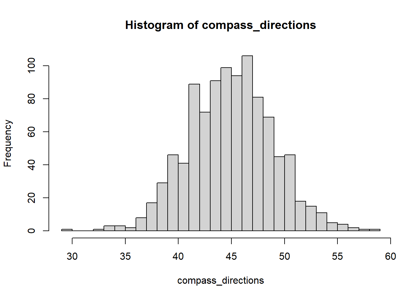

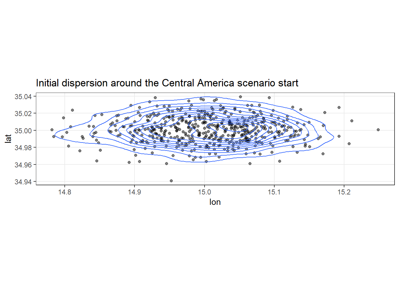
Initial positions are created by taking some plausible position and drawing points from a bivariate normal distribution dispersed on some uncertainty in longitude and latitude. The paper left out is the fact that we need a covariance matrix for this: I assembled one using an assumed correlation of 0.

#generate uncertainty around initial fix

generate_initial_distribution <- function(init_lat, init_lon, sigma_lat, sigma_lon, n, correlation=0){
  
  lat_sigma_deg <- sigma_lat / 60
  lon_sigma_deg <- sigma_lon / (60 * cos(init_lat * pi / 180))
  
  cov_matrix <- matrix(c(lat_sigma_deg^2, correlation*lat_sigma_deg*lon_sigma_deg,
                         correlation*sigma_lat*lon_sigma_deg,lon_sigma_deg^2), 
                       nrow = 2)
  
  samples <- mvrnorm(n, mu = c(init_lat, init_lon), Sigma = cov_matrix)
  
  tibble(lat = samples[,1],
         lon = samples[,2])
}

Here’s what that looks like visually. What we’re doing is, given a last location estimate and reasonable measures of how wrong this can be, sample a set number of points. There will comparatively be a much higher density of points towards the middle, but values towards the outsides are plausible as well, just not as common.

The whole crux of the Bayesian approach is to:

• use evidence (in this case historical testimony) to come up with likely scenarios

• draw values for those scenarios from probability distributions of plausible numbers

• simulate thousands of independent trials for a given scenario

• count the number of times a scenario ends up in a given grid

Stone details three scenarios the team give credence to. We’ll explore them all briefly and run them to get a better understanding of how the above loop works.

Central America Scenario

The first scenario is named the “Central America” scenario, which builds on the fact that Captain Herndon onboard the Central America relayed a fix obtained through celestial navigation to the nearby El Dorado. Establishing latitude from a celestial body is just a matter of measuring how high it is, but establishing longitude also depends on having an accurate clock on board, which increases uncertainty. (P.S. this is the reason navies had handsome prize funds for clock makers in the 18th century.)

The Central America was powerless for the duration of this scenario, meaning it was drifting. Drift at sea for a ship is a function of the sea currents and the wind acting on the ship structure. We also get all these values from the paper, (and I took some liberty to simplify: technically there is a wind component to currents too that acts independently of geostrophic current, but I combined these into one sea drift normal distribution.)

#initial params for Central America scenario
start_lon <- -77.166667
start_lat <- 31.416667
direction <- 45  #degrees i.e. NE
time_steps <- 13 #hours

uncertainty_lat <- 0.9
uncertainty_lon <- 3.9

n_sims <- 10000

Here are all the pieces wrapped up: we generate n_sims number of draws from the position as our start. The for loop iterates through each row, randomly draws up a drift velocity D, which we then feed to our simulate_drift function.

The one thing that I couldn’t find specified in the paper was the average range of wind speeds. I know they can be pretty high in a hurricane, but we are talking the average over 13 hours here, so I went with a mean of 30 knots and a standard deviation of 15 knots.

#run all pieces in a loop
df <- data.frame()

start_points <- generate_initial_distribution(start_lat, start_lon, uncertainty_lat, uncertainty_lon, n_sims)

for(i in 1:nrow(start_points)){
  lat <- start_points[i, "lat"]$lat
  lon <- start_points[i, "lon"]$lon
  
  #drift: D = (V + fW)
  D <- rnorm(n=1, mean=1.35, sd=0.2) + (rnorm(n=1, mean= 30, sd=15) * 0.03)
  
  sim <- simulate_drift(lon, lat, direction, D, time_steps) |> 
    mutate(run = i)
  df <- bind_rows(df, sim)
  }

And just in case it’s still not clear what simulate drift is doing, here’s the first 10 runs plotted:

df %>% 
  filter(run <= 10) %>% 
  ggplot()+
  geom_point(aes(x=lon, y=lat, group=run, colour=step))+
  geom_line(aes(x=lon, y=lat, group=run, colour=step))+
  coord_map()+
  theme_bw()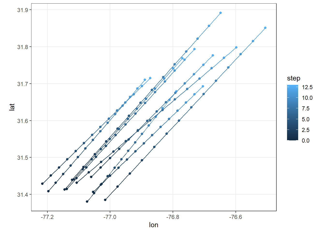

The next bit is just some processing. We only keep the final positions (where we assume the ship sank, which in this scenario are at hour 13), and assign the individual points into lon/lat bins. Then we count the number of points in each of these bins, and the Monte Carlo derived probability of the Central America being in this bin is the count divided by n_sims.

data <- df %>% 
  mutate(final = if_else(step==13, T, F)) |> 
  #only keep final positions
  filter(final) %>% 
  mutate(
    lon_bucket = floor(lon / grid_size_deg_lon) * grid_size_deg_lon,
    lat_bucket = floor(lat / grid_size_deg_lat) * grid_size_deg_lat
  )

# Count the number of points in each grid cell
central_america_scenario <- data %>%
  group_by(lon_bucket, lat_bucket) %>%
  summarise(count = n(),
            p = count/n_sims) %>%
  ungroup()

What we end up with is the following probability map. This should be roughly analogous to figure 3 in the paper.

# Plot the heatmap with lat/lon axes
ggplot(central_america_scenario, aes(x = lon_bucket, y = lat_bucket)) +
  geom_tile(aes(fill = p), color = "white") +
  scale_fill_gradient(low = "white", high = "red") +
  geom_point(aes(x=start_lon, y=start_lat))+
  annotate("text", x=start_lon, y=start_lat, label = "Herndon: Start Point", hjust=-0.05)+
  geom_point(aes(x=-76.833333, y=31.666667), shape=4)+
  annotate("text", x=-76.833333, y=31.666667, label = "Marine", vjust=1)+
  geom_point(aes(x=-76.216667, y= 31.916667), shape=4)+
  annotate("text", x=-76.216667, y=31.916667, label = "Ellen", vjust=1)+
  coord_map() +
  labs(
    x = "Longitude",
    y = "Latitude",
    fill = "Density"
  ) +
  theme_minimal()+
  scale_x_continuous(labels = function(x) sapply(x, convert_to_deg_min), limits=c(-77.2, -76)) + 
  scale_y_continuous(labels = function(y) sapply(y, convert_to_deg_min), limits = c(31.4, 32))+
  labs(title = "Monte Carlo Probabilities for Central America Scenario",
       caption = "Based on Stone, 1992.",
       fill = 'Probability')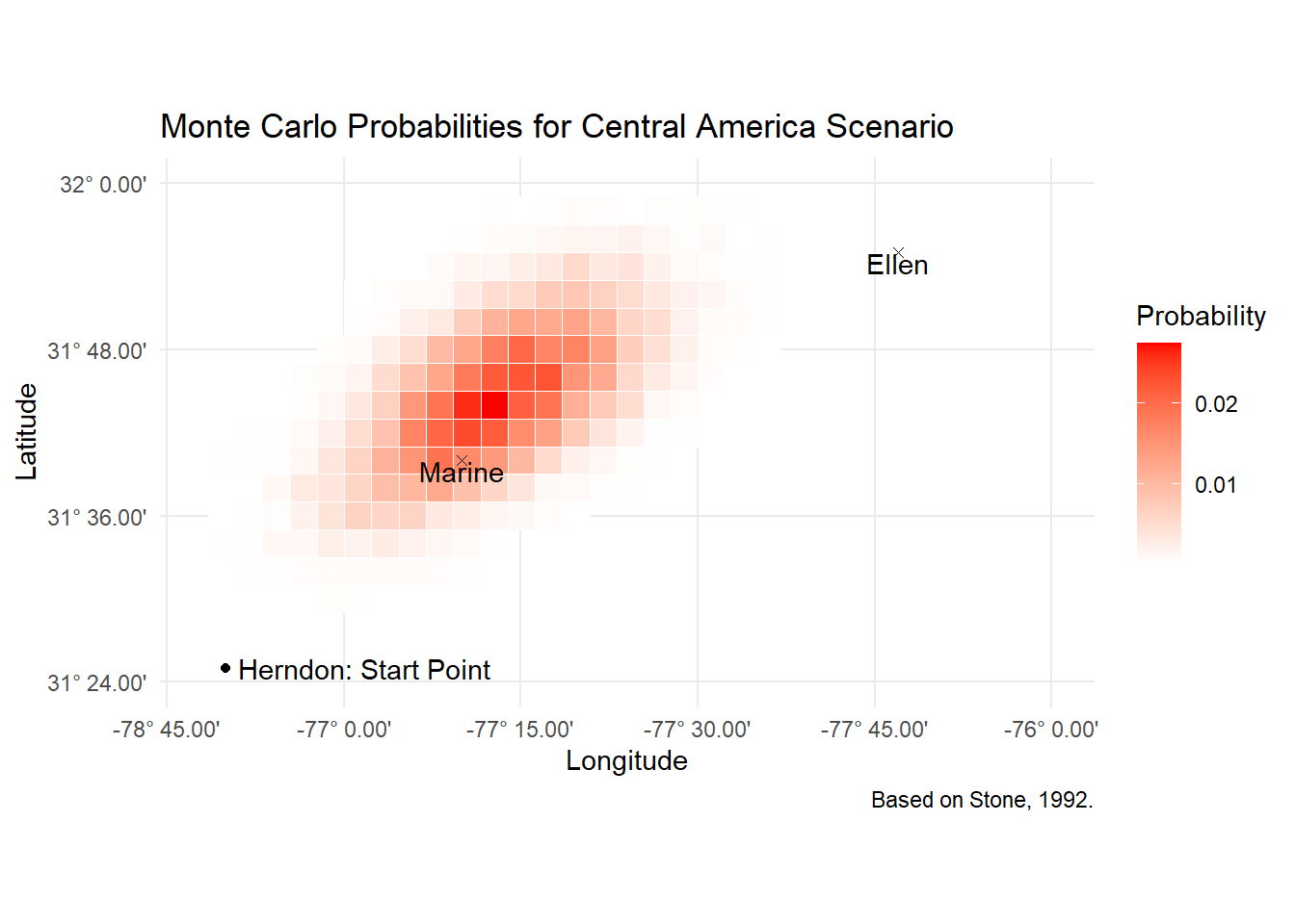

It’s the exact same approach for the other two scenarios.

Ellen Scenario

The Ellen scenario builds on the fact that the Norwegian bark Ellen picked up survivors at 31° 55’N, 76° 13’W 12 hours after the sinking. Again assuming some error for the fact that this is a fix derived from celestial navigation, we populate n_sim points, only this time we need to drift in reverse. This is easily accomplished by turning velocity negative. We also do away with leeway drift, since wind does not impart a meaningful drift to people in the water.

#initial params for Ellen scenario
start_lon <- -76.216667
start_lat <- 31.916667
direction <- 45  #degrees i.e. NE
time_steps <- 12 #hours

uncertainty_lat <- 0.9
uncertainty_lon <- 5.4

n_sims <- 10000

df <- data.frame()

start_points <- generate_initial_distribution(start_lat, start_lon, uncertainty_lat, uncertainty_lon, n_sims)

for(i in 1:nrow(start_points)){
  lat <- start_points[i, "lat"]$lat
  lon <- start_points[i, "lon"]$lon
  
  #drift: D = (V + fW)
  D <- rnorm(n=1, mean=1.2, sd=0.3) # person has no leeway
  D = D * -1 #we're drifting a person backwards
  
  sim <- simulate_drift(lon, lat, direction, D, time_steps) |> 
    mutate(run = i)
  df <- bind_rows(df, sim)
  }

data <- df %>% 
  mutate(final = if_else(step==12, T, F)) %>%
  #only keep final positions
  filter(final) %>% 
  mutate(
    lon_bucket = floor(lon / grid_size_deg_lon) * grid_size_deg_lon,
    lat_bucket = floor(lat / grid_size_deg_lat) * grid_size_deg_lat
  )

# Count the number of points in each grid cell
ellen_scenario <- data %>%
  group_by(lon_bucket, lat_bucket) %>%
  summarise(count = n(),
            p = count/n_sims) %>%
  ungroup()

ggplot(ellen_scenario, aes(x = lon_bucket, y = lat_bucket)) +
  geom_tile(aes(fill = p), color = "white") +
  scale_fill_gradient(low = "white", high = "red") +
  geom_point(aes(x=start_lon, y=start_lat), size=2, shape=4)+
  geom_point(aes(x=-76.833333, y=31.666667), shape=4)+
  geom_point(aes(x=-76.216667, y= 31.916667), shape=4)+
  annotate("text", x=-76.833333, y=31.666667, label = "Marine", vjust=1.2)+
  annotate("text", x=-76.216667, y=31.916667, label = "Ellen", vjust=1.5)+
  coord_map() +
  labs(
    x = "Longitude",
    y = "Latitude",
    fill = "Density"
  ) +
  theme_minimal()+
  scale_x_continuous(labels = function(x) sapply(x, convert_to_deg_min), limits=c(-77.2, -76)) + 
  scale_y_continuous(labels = function(y) sapply(y, convert_to_deg_min), limits = c(31.4, 32))+
  labs(title = "Monte Carlo Probabilities for Ellen Scenario",
       caption = "Based on Stone, 1992.",
       fill = 'Probability')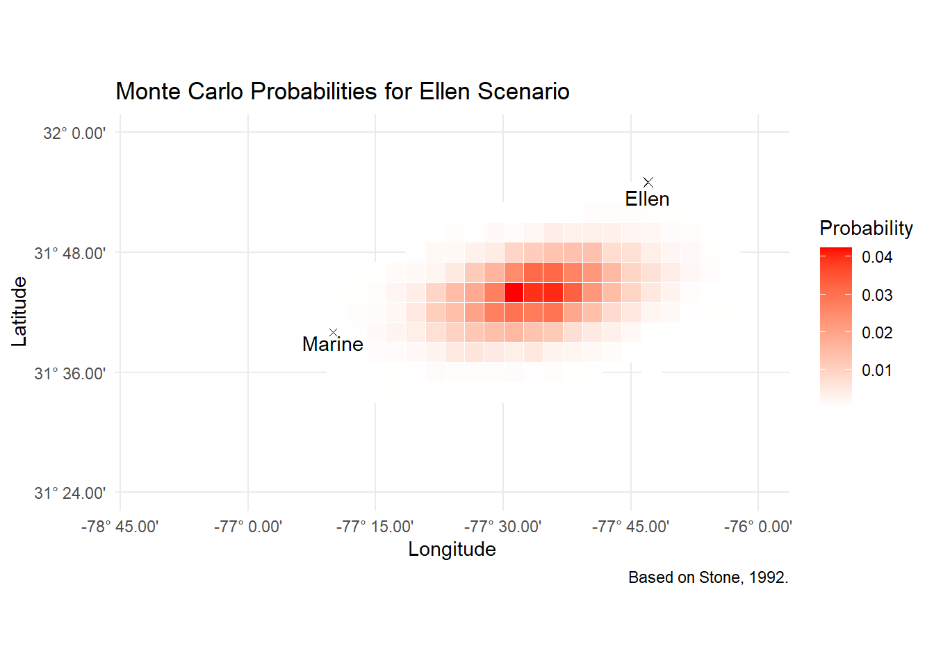

Marine Scenario

Finally, the Marine scenario involves the sighting of the SS Central America by another ship, the Marine. Interestingly, the uncertainty here is larger circular. Some 36 hours had elapsed since the Marine last calculated it’s position celestially, meaning the position given was estimated by the crew using dead reckoning. But unlike celestial navigation, where it’s easier to be off in one direction than the other, with dead reckoning it’s just as likely all round. This subtle nuance really underlines the advantages of probabilistic techniques like these, you can nest many situations, with each having tailored probability distributions for their parameters.

The uncertainty on the exact geometry of the sighting is modelled through a uniform distribution of [1, 6] for distance and [7, 127] for angle. The resulting points then were drifted as before.

#initial params for Marine scenario

start_lon <- -76.833333
start_lat <- 31.666667

uncertainty_lat <- 9
uncertainty_lon <- 9

direction <- 45  #degrees i.e. NE
time_steps <- 7 #hour

n_sims <- 10000

start_points <- generate_initial_distribution(start_lat, start_lon, uncertainty_lat, uncertainty_lon, n_sims)

start_points%>% 
  ggplot(aes(x=lon, y =lat))+
  geom_point(alpha=0.4)+
  geom_density_2d()+
  theme_bw()+
  labs(title="What the Marine's initial start points look like",
       subtitle = 'Notice how this distirbution is more round as opposed to Eliptical')

df <- data.frame()

for(i in 1:nrow(start_points)){
  lat <- start_points[i, "lat"]$lat
  lon <- start_points[i, "lon"]$lon
  
  s <- runif(n=1, min=1, max=6) 
  theta <- runif(n=1, min = 7.5, max = 127.5)
  
  estimated_central_america_pos <- simulate_drift(start_lon = lon, start_lat = lat, direction = theta, speed = s, time_steps=1) %>% 
    filter(step==1)
  
  D <- rnorm(n=1, mean=1.3, sd=0.2) + (rnorm(n=1, mean= 30, sd=15) * 0.03)
  drifted <- simulate_drift(estimated_central_america_pos$lon,
                            estimated_central_america_pos$lat,
                            speed =D,
                            direction = direction,
                            time_steps = time_steps) %>% 
    mutate(run = i)
  
  df <- bind_rows(df, drifted)
  }

data <- df %>% 
  mutate(final = if_else(step==7, T, F)) |> 
  #only keep final positions
  filter(final) %>% 
  mutate(
lon_bucket = floor(lon / grid_size_deg_lon) * grid_size_deg_lon,
    lat_bucket = floor(lat / grid_size_deg_lat) * grid_size_deg_lat
  )

# Count the number of points in each grid cell
marine_scenario <- data %>%
  group_by(lon_bucket, lat_bucket) %>%
  summarise(count = n(),
            p = count/n_sims) %>%
  ungroup()

ggplot(marine_scenario, aes(x = lon_bucket, y = lat_bucket)) +
  geom_tile(aes(fill = p), color = "white") +
  scale_fill_gradient(low = "white", high = "red") +
  geom_point(aes(x=start_lon, y=start_lat), size=2, shape=4)+
  geom_point(aes(x=-76.833333, y=31.666667), shape=4)+
  geom_point(aes(x=-76.216667, y= 31.916667), shape=4)+
  geom_point(aes(x= -77.166667, y=31.416667))+
  annotate("text", x=-76.833333, y=31.666667, label = "Marine", vjust=1.2)+
  annotate("text", x=-76.216667, y=31.916667, label = "Ellen", vjust=1.5)+
  coord_map() +
  labs(
    x = "Longitude",
    y = "Latitude",
    fill = "Density"
  ) +
  theme_minimal()+
  scale_x_continuous(labels = function(x) sapply(x, convert_to_deg_min), limits=c(-77.2, -76)) + 
  scale_y_continuous(labels = function(y) sapply(y, convert_to_deg_min), limits = c(31.4, 32.2))+
  labs(title = "Monte Carlo Probabilities for Marine Scenario",
       caption = "Based on Stone, 1992.",
       fill = 'Probability')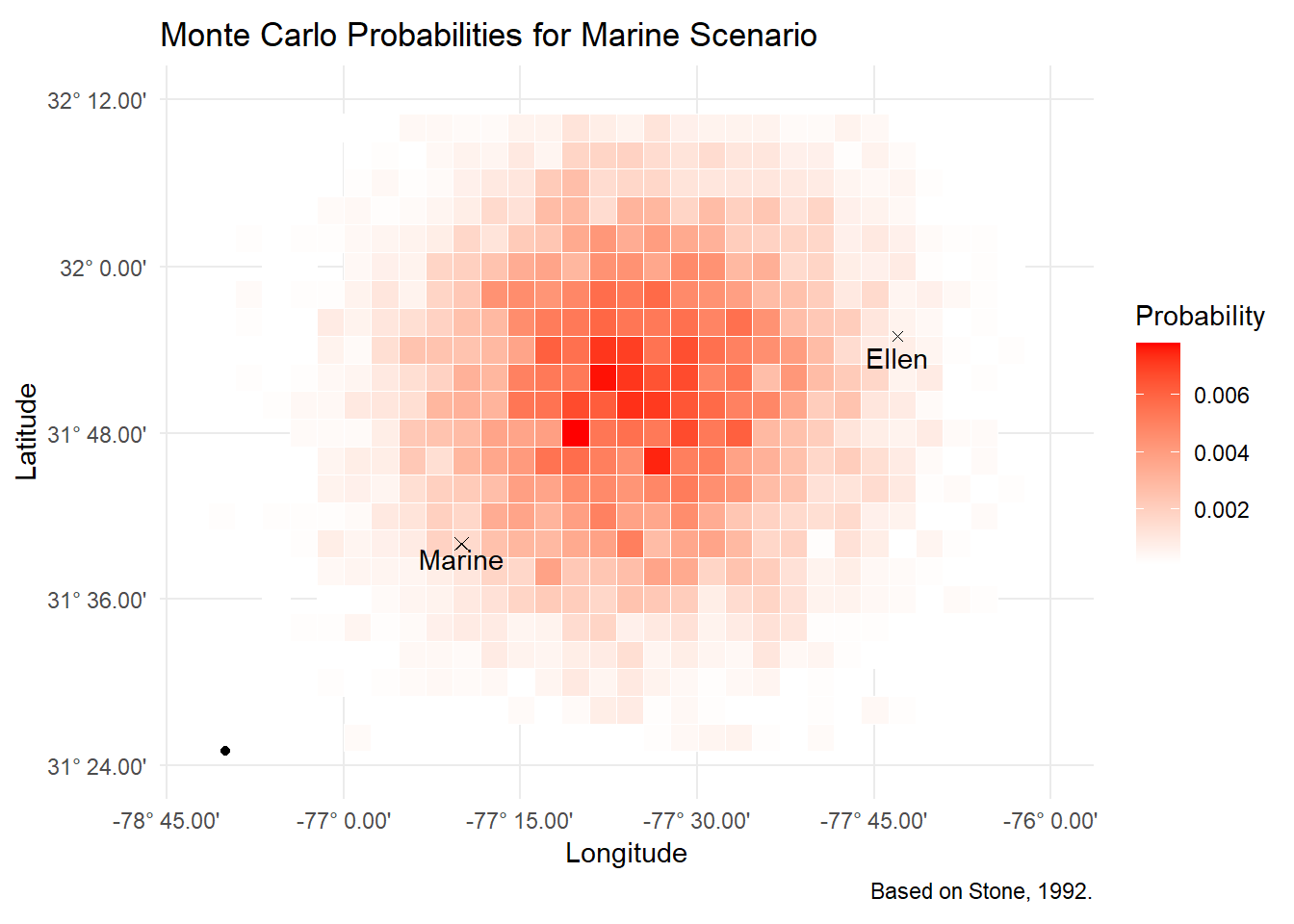

Composite Probability

The final piece lies in assembling the probability maps for the three separate scenarios we have together, something which Stone calls a ‘composite probability map’. Again, the neat thing here is we can assign different weights to different scenarios to reflect how plausible we believe they are. Following discussions, the teams settled on the weighting scheme:

#subjective weight scheme
tibble(scenario = c("Central America", "Ellen", "Marine"),
       weight = c(23, 72, 5))

## # A tibble: 3 × 2
##   scenario        weight
##   <chr>            <dbl>
## 1 Central America     23
## 2 Ellen               72
## 3 Marine               5

The end probability of a cell is then the weighted probability of all three scenarios. I achieve this by joining all three scenarios together. Some cells only have probabilities from 1 scenario. Here we set the p of other scenarios to 0.

## Combine scenarios and weight

central_america_scenario <- central_america_scenario %>% 
  mutate(weight = 0.23) %>% 
  rename(count_scen1 = count,
         p_scen1 = p,
         weight_scen1 = weight)

ellen_scenario <- ellen_scenario %>% 
  mutate(weight = 0.72)%>% 
  rename(count_scen2 = count,
         p_scen2 = p,
         weight_scen2 = weight)

marine_scenario <- marine_scenario %>% 
  mutate(weight = 0.05)%>% 
  rename(count_scen3 = count,
         p_scen3 = p,
         weight_scen3 = weight)

composite_p <- central_america_scenario %>% 
  full_join(ellen_scenario, by = c("lon_bucket", "lat_bucket")) %>% 
  full_join(marine_scenario, by = c("lon_bucket", "lat_bucket"))%>%
  mutate_all(~ replace_na(., 0)) %>% 
  mutate(weighted_p = (count_scen1 * weight_scen1 + count_scen2 * weight_scen2 + count_scen3 * weight_scen3)/n_sims)

What we end up with is something like this:

composite_p %>% 
  sample_n(5)

## # A tibble: 5 × 12
##   lon_bucket lat_bucket count_scen1 p_scen1 weight_scen1 count_scen2 p_scen2
##        <dbl>      <dbl>       <int>   <dbl>        <dbl>       <int>   <dbl>
## 1      -76.4       32.0           0  0              0              0  0     
## 2      -76.4       31.9           2  0.0002         0.23           0  0     
## 3      -76.0       32.1           0  0              0              0  0     
## 4      -76.4       31.6           0  0              0              1  0.0001
## 5      -77.1       32.0           0  0              0              0  0     
## # ℹ 5 more variables: weight_scen2 <dbl>, count_scen3 <int>, p_scen3 <dbl>,
## #   weight_scen3 <dbl>, weighted_p <dbl>

And when you plot it:

ggplot(composite_p, aes(x = lon_bucket, y = lat_bucket)) +
  geom_tile(aes(fill = weighted_p), color = "white") +
  scale_fill_gradient(low = "white", high = "red") +
  geom_point(aes(x=-76.833333, y=31.666667), shape=4)+
  geom_point(aes(x=-76.216667, y= 31.916667), shape=4)+
  geom_point(aes(x= -77.166667, y=31.416667))+
  annotate("text", x=-76.833333, y=31.666667, label = "Marine", vjust=1.2)+
  annotate("text", x=-76.216667, y=31.916667, label = "Ellen", vjust=1.5)+
  annotate("text", x= -77.166667, y=31.416667, label = "Herndon", vjust=1.5)+
  coord_map() +
  labs(
    x = "Longitude",
    y = "Latitude",
    fill = "Density"
  ) +
  theme_minimal()+
  scale_x_continuous(labels = function(x) sapply(x, convert_to_deg_min)) + 
  scale_y_continuous(labels = function(y) sapply(y, convert_to_deg_min))+
  labs(title = "Composite Monte Carlo Probability for Location of USS Central America",
       fill = 'Probability')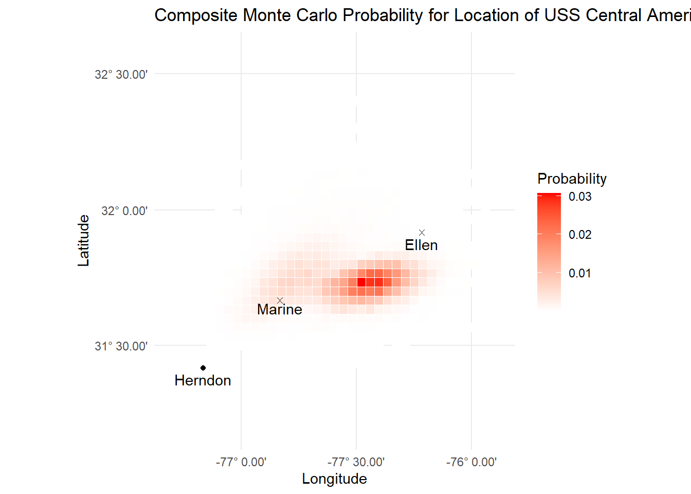

Annoyingly, this final composite map looks a bit different than the one in the paper, which means I’ve gone astray slightly, but I’ll stick with it since the Central America has already been found. But more importantly, there’s still much more to Bayesian methods than this.

Bayesian Search Magic

In some ways, the composite probability map above is just the start which you can treat as your prior distribution. Given we have some detection tool, be it sonar or an eyeball, that given a cell and a wreck has, let’s say, an 80% probability of detecting the wreck, we can update the map iteratively with this new information. What we get back is a constantly updating probability map based on the new information coming in after searching each cell.

The truly astounding thing about this approach is that if we search a high probability cell with an instrument with a high but not perfect probability of detection, that cell drops in probability but is not discounted entirely. This becomes clear in the graphic in search numbers 55 to 70, where the initial high density probability that was first searched, becomes the most probable again after searching 50 other cells.

An unfolding Bayesian search based on a detection probability of 0.8.

In fact, most of the initial search area is re-searched again before expanding outwards to the much lower probability cells on the outside.

The sonar used in the search by Thompson and the team had an estimated 99% detection probability, provided the wreck was in a sweet spot 500 to 2,500 meters within the sensor. Any closer than 500 meters, and reverberation from the seafloor would drop the detection probability to 0.9. Any further than 2.5km, and the detection probability would plummet to close to zero.

The rest of the paper also details some other fascinating operational research topics, like needing to devise a path that maximises traversing high probability cells most efficiently (since high probability cells are not necessarily close together and are often between much lower probability cells.

In the end, Central America was found in a relatively low probability cell, roughly half way between it’s last reported position and where the Marine sighted it, close to the higher probability left cluster. I think it must be emphasised that this wasn’t a defeat for the methodology in any meaningful sense. It is likely that without this approach that cell would probably not have been searched at all, and in the Bayesian sense low probability does not mean impossibility. Indeed, this is something another mariner knew well:

(and yes, I did put Pirates of the Carribean on as I was writing this)

Dr. Lawrence Stone continued polishing this work, developing SAROPS, a Bayesian Search inspired computer system that the US Coast Guard uses to respond to emergencies at sea and founding Metron, a science consultancy with some impressive projects, including finding Air France 447.

As to the Central America, the Columbus America Discovery Group did manage to salvage some of the gold, but has been stuck in a legal quagmire since. Thompson was jailed in 2015 for contempt of court, after he said he could not remember where 500 coins he raised from the wreck were. He remains in jail to this day. Coincidentally in the process of writing this, I found out National Geographic is airing a three part series on the saga. There’s also a highly acclaimed book by Gary Kinder on the nuances of the search which is well worth a read.

References

Search for the SS Central America: Mathematical Treasure Hunting, Stone, 1992

KINDER, G. (2018) Ship of gold in the deep blue sea: The history and discovery of the world’s Richest Shipwreck. GROVE.